Supervised Learning

Linear regression with one variable

Target : From a dataset (red points), we want to find a general method to automatically get an hypothesis function ${h_\theta(x)=\theta_0+\theta_1x}$ (blue line) that fit as well our points to predict new incomming data.

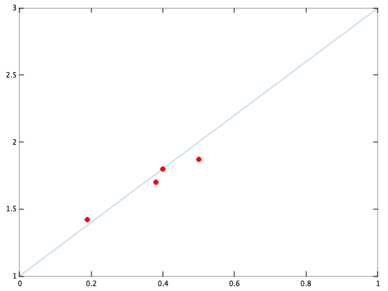
Solution : Find a cost function $J(\theta)$ of parameter $(\theta_0,\theta_1)$ with $\theta$ that minimise $J$

$$ J(\theta_0,\theta_1) = \dfrac{1}{2m} \sum_{i=1}^m (h_\theta(x^{(i)})-y^{(i)})^2 $$

where $m$ the number of training sets

Gradient descent algorithm to automatically compute and find $\theta$

$$ \theta_j := \theta_j - \alpha \dfrac{\partial}{\partial \theta_j} J(\theta_j), j=[0,1] $$

Warning : All $\theta_j$ are simultaneously updated until reach convergence

Multivariate linear regression

We hold more than one variable. Hence our hypothesis function is now : ${h_\theta(x)=\theta_0+\theta_1x_1+\dots+\theta_nx_n}$

To simpplify expression we define $x_0=1$, $\theta$ is a $(n+1)$ dimensional vector

Vectorization of our hypothesis $\rightarrow$ ${h_\theta(X)=\theta^TX}$

Cost function still the same

$$J(\theta) = \dfrac{1}{2m} \sum_{i=1}^m (h_\theta(x^{(i)})-y^{(i)} )^2$$

Gradient descent : Method to solve for $\theta$ iteratively

General form expression. $n$ the number of features in training sets $$ \theta_j := \theta_j - \alpha \dfrac{\partial}{\partial \theta_j} J(\theta_j), j=[0, \dots,n] $$

• Simplification

When $j=0$ : $$ \theta_0 := \theta_0 - \alpha \dfrac{\partial}{\partial \theta_0} [\dfrac{1}{2m} \sum_{i=1}^m (h_\theta(x^{(i)})-y^{(i)} )^2] $$ $$ \theta_0 := \theta_0 -\dfrac{\alpha}{\cancel{2}m}*\cancel{2} \sum_{i=1}^m (h_\theta(x^{(i)})-y^{(i)})x_0^{(i)} $$

We repeat this process when $j=1$, $j=2$, $\ldots$ More generally by induction we finally get :

$$ \theta_j := \theta_j -\dfrac{\alpha}{m}\sum_{i=1}^m (h_\theta(x^{(i)})-y^{(i)})x_j^{(i)} $$

• Optimisation : Feature scaling & Mean normalisation

When difference between values of features are too large, they cause that gradient descent run slowly to find the global optimum $\theta$. Instead of taking them as they are, we make a transformation to hold them at the same scale. This ensure that gradient descent will converge more faster. From training set : $(a_i,b_i,\dots,y_i)$

$a_i \leftarrow \frac{a_i - \mu_i}{S_i}$ where $\mu_i$ is the mean of $a_i$ other the set and $S_i$ the standard deviation or simply range $(max_{value} - min_{value})$.

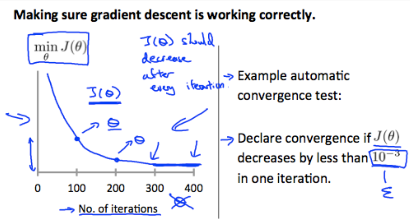
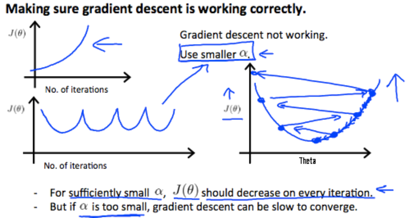
• Learning rate

_	_

Normal Equation : Method to solve for $\theta$ analytically $$ \theta = (\mathbf{X}^\top \mathbf{X})^{-1}\mathbf{X}^\top y $$ Where $X$ is the design matrix

$$ \mathbf{X} = \left( \begin{array}{ccc} — & [x^{(0)}]^\top & — \\ — & [x^{(1)}]^\top & — \\ — & \ldots & — \\ — & [x^{(m)}]^\top & — \\ \end{array} \right) $$

• GDA vs NE

Gradient Descent	Normal Equation
Need to choose $\alpha$	No need to choose $\alpha$
Needs many iterations	No needs many iterations
$O(kn^2)$	$O(n^3)$, need to calculate $(\mathbf{X}^\top \mathbf{X})^{-1}$
Works well when n is large	Slow if n is very large ($n>10^4$)

Logistic Regression

WIP…